


Tufte Handout
A wide-margin lecture handout with sidenotes in the style of Edward Tufte.
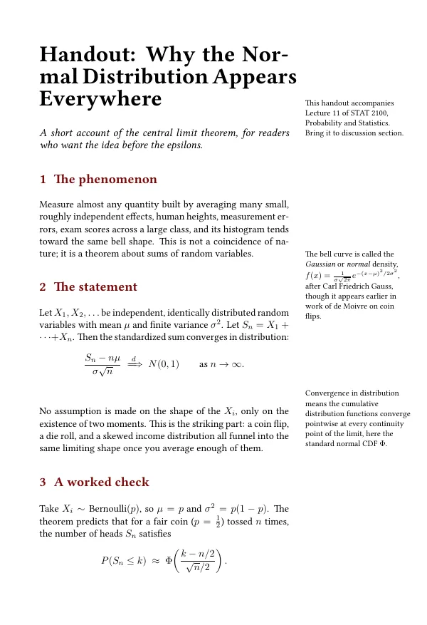
main.tex
\documentclass[11pt]{article}
\usepackage[paperwidth=6.5in,paperheight=9.5in,
  left=0.6in,right=2.1in,top=0.7in,bottom=0.8in,marginparwidth=1.6in,marginparsep=0.25in]{geometry}
\usepackage{amsmath,amssymb}
\usepackage{mathtools}
\usepackage{libertine}
\usepackage{xcolor}
\usepackage{marginnote}
\usepackage{titlesec}

\definecolor{accent}{HTML}{7A0C0C}

\titleformat{\section}{\normalfont\Large\bfseries\color{accent}}{\thesection}{0.6em}{}
\titlespacing*{\section}{0pt}{1.2em}{0.6em}

\newcommand{\sidenote}[1]{\marginnote{\footnotesize #1}}

\setlength{\parindent}{0pt}
\setlength{\parskip}{0.6em}
\pagestyle{empty}

\begin{document}

{\Huge\bfseries Handout: Why the Normal Distribution Appears Everywhere}
\sidenote{This handout accompanies Lecture 11 of STAT 2100, Probability
and Statistics. Bring it to discussion section.}

\bigskip
{\large\itshape A short account of the central limit theorem, for readers
who want the idea before the epsilons.}

\section{The phenomenon}

Measure almost any quantity built by averaging many small, roughly
independent effects, human heights, measurement errors, exam scores
across a large class, and its histogram tends toward the same bell shape.
This is not a coincidence of nature; it is a theorem about sums of random
variables.\sidenote{The bell curve is called the \emph{Gaussian} or
\emph{normal} density, $f(x) = \frac{1}{\sigma\sqrt{2\pi}}
e^{-(x-\mu)^2/2\sigma^2}$, after Carl Friedrich Gauss, though it appears
earlier in work of de Moivre on coin flips.}

\section{The statement}

Let $X_1, X_2, \ldots$ be independent, identically distributed random
variables with mean $\mu$ and finite variance $\sigma^2$. Let
$S_n = X_1 + \cdots + X_n$. Then the standardized sum converges in
distribution:
\[
  \frac{S_n - n\mu}{\sigma\sqrt{n}} \;\xRightarrow{\ d\ }\; N(0, 1)
  \qquad \text{as } n \to \infty.
\]
\sidenote{Convergence in distribution means the cumulative distribution
functions converge pointwise at every continuity point of the limit,
here the standard normal CDF $\Phi$.}

No assumption is made on the shape of the $X_i$, only on the existence of
two moments. This is the striking part: a coin flip, a die roll, and a
skewed income distribution all funnel into the same limiting shape once
you average enough of them.

\section{A worked check}

Take $X_i \sim \text{Bernoulli}(p)$, so $\mu = p$ and
$\sigma^2 = p(1-p)$. The theorem predicts that for a fair coin
($p = \tfrac12$) tossed $n$ times, the number of heads $S_n$ satisfies
\[
  P(S_n \le k) \;\approx\; \Phi\!\left(\frac{k - n/2}{\sqrt{n}/2}\right).
\]
\sidenote{This is the de Moivre-Laplace approximation, the historical
first case of the central limit theorem, proved in 1733.}
For $n = 100$ the exact probability $P(S_{100} \le 45)$ from the binomial
distribution is about $0.184$, while the normal approximation gives
$\Phi(-1) \approx 0.159$; a continuity correction closes most of the gap.

\section{Why it matters}

The central limit theorem is the reason confidence intervals, control
charts, and standard errors all lean on the normal distribution by
default. It is also why sample means, not individual measurements, are
the workhorse of applied statistics: averaging suppresses idiosyncratic
noise and reveals the shared limiting shape underneath.

\end{document}
In the app: open the New Project gallery, install the Coursework pack under "Get more templates", and this template appears with a live preview and one-click project creation. Compilation runs locally on the bundled engine.